
Most businesses use Google Sheets to either display or share data. However, if you can tap into the power of Google Sheets functions, they can do wonders for your business.
Using Google Sheets functions, you can work more efficiently and keep data organized. What’s more, you can even use Google Sheets functions to perform data analytics and make effective decisions.
In this way, you can increase revenue by increasing the accuracy of your data, and making it easier to access and use.
In this article, we’re sharing our top 10 spreadsheet formulas that are sure to turn your business around. Not only will you be saving time with these hacks, you will also ensure that your data is neat, accessible and error-free.
Here they are!
IF and IFS
Contents
The IF and IFS functions are evidently two of the most popular and widely-used Google Sheets functions. They were basically created to perform an action based on one or more conditions, but their applications are limitless!
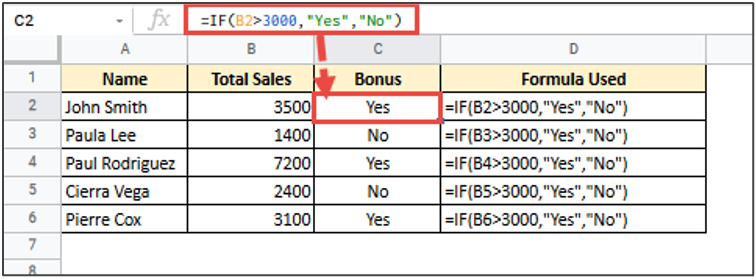
For example, say you have a list of employee sales data and you want to find out which employees deserve a bonus.
You can use the IF function to check if their sales are over a given amount. For example, if Sales total is more than $3,000 then you can specify the IF function to display a “Yes”, and if not, then you can specify the function to display a “No”, as follows:
Displaying a simple “Yes” or “No” is helpful enough, but you can go one step further and even calculate the bonus based on their Sales. This means you can insert a formula into the IF statement, instead of just specifying a text to display, as shown below:
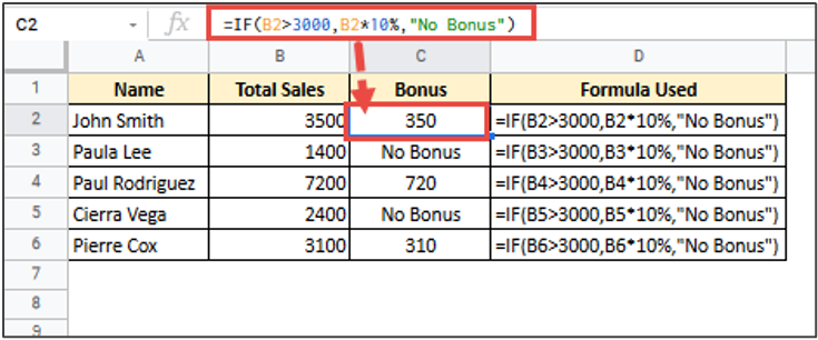
In the above image, we specified that if the employee’s sales is more than $3,000, the employee gets a 10% bonus on sales made. Otherwise, the employee gets “No Bonus”.
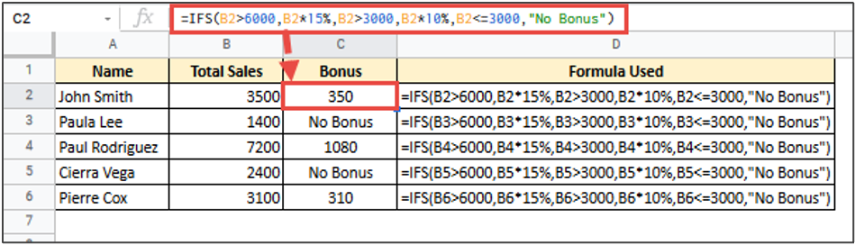
If you need to specify more than one condition, the IFS function will be more suitable. So, for example, you can specify a 10% bonus for sales higher than $3,000, and a 15% bonus for sales higher than $6,000, as shown in the image below:
COUNTIF
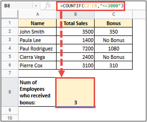
The COUNTIF function can help you count cells in a range that satisfy a given condition. For example, if you want to count how many employees received a bonus in the previous example, you could simply use the COUNTIF function as follows:
SUMIF and SUMIFS
SUMIF adds all cells that meet certain criteria
Similar to the COUNTIF function, the SUMIF and SUMIFS functions are basically just a combination of the SUM and IF/IFS functions. Both these functions basically add all cells that meet one (or more) criteria.
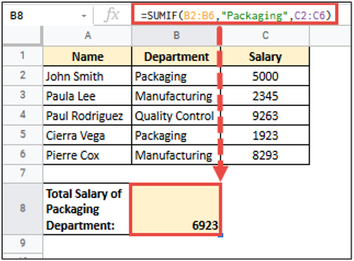
For example, if you want to find out total salary of employees belonging to a given department (say “Packaging”) you can use the SUMIF function as follows:
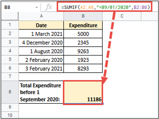
You could also use this function to find out the total company expenditure before a given date, as follows:
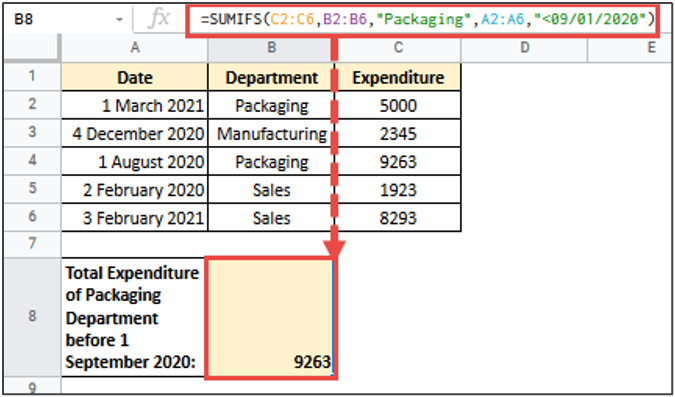
Like the IFS function the SUMIFS function is used when you want to consider more than one condition in finding a sum. So in the above example, if you want to find out total expenditure on raw materials that were made by the Packaging department before a given date, you can use the SUMIFS function as follows:
VLOOKUP
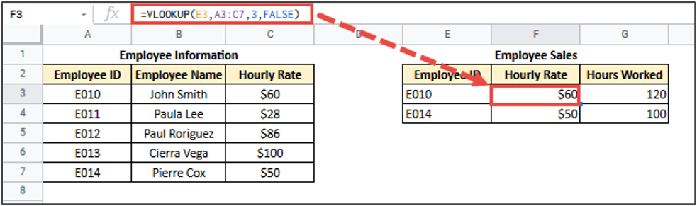
The word VLOOKUP is short for ‘Vertical Lookup’. This function allows you to search for a certain key value in a column and returns a corresponding value in the same row of a different column.
For example, you might have one table that contains employee information and another that contains information about employee sales, as shown below:
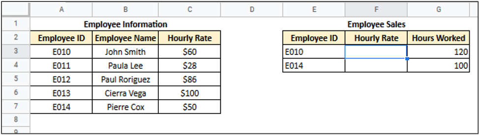
If you want to know the Hourly Rate for each employee in the second table, you can pull this information form the first table with the VLOOKUP function as shown below:
IFERROR
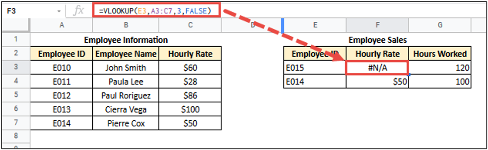
The VLOOKUP function works great, as long as the key value you’re looking for actually exists in the lookup table. If it doesn’t then the VLOOKUP function simply gives you an error message, as shown below:
The IFERROR function allows you to handle error messages like these. So, if you anticipate that a certain function or formula might return an error, you could use the IFERROR function to specify what to do in such cases.
For example, when a VLOOKUP function returns an error after not having found a search key, the IFERROR function could return a text that says “Not found”, as shown below:
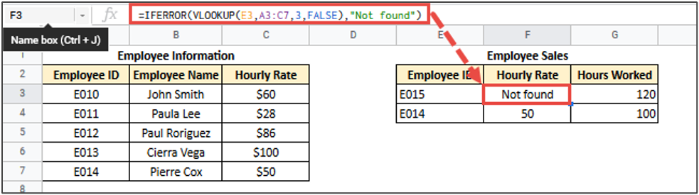
It’s important to remember here that the IFERROR function treats all errors the same way. This means it cannot differentiate between a #N/A error and #NUM! error, or any other error string.
IMPORTRANGE
VLOOKUP works great on its own when your lookup table is on the same sheet or a different sheet within the same workbook.
However, if you need to lookup a value from a table that is in a separate workbook, you will need to use the IMPORTRANGE function.
The IMPORTRANGE function is used to import values from cells in another spreadsheet into your current spreadsheet. To use it, all you need to do is specify the URL of the workbook, the sheet name and a reference to the range of cells you want to access. That is, of course, provided you have access permission to the particular workbook.
For example, if the employee information lookup table (that we discussed before) were located in a different worksheet, we would need to include the IMPORTRANGE function within the VLOOKUP formula to access it as follows:

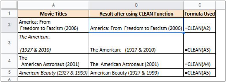
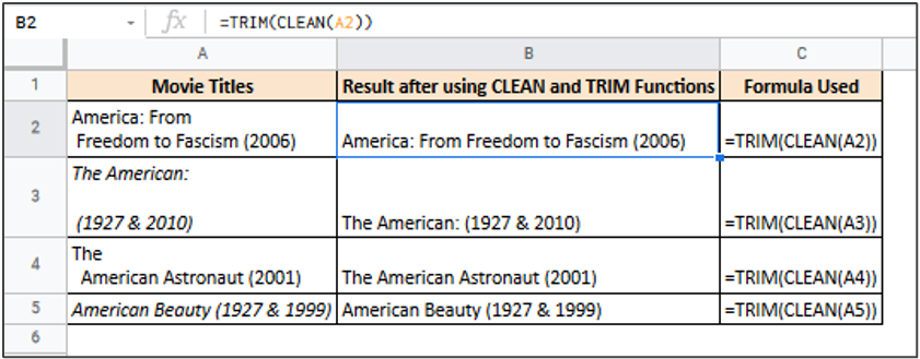
CLEAN and TRIM
When you import data from an outside source, you are often faced with the annoying task of cleaning up the data. This cleaning up task often consists of removing extra spaces at the beginning or end of cells.
Moreover, some cells might contain special characters that are hidden in the imported text. Try performing operations on these cells and you’ll find results far from what you expected.
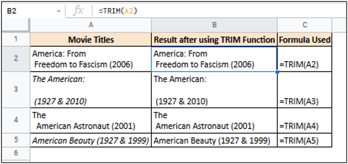
For example, consider the data shown below:

The TRIM function can be used here to remove all the leading and trailing space characters (“ “) from text. If there are extra spaces between words, then it removes the extras and leaves just a single space.
Sometimes what might look like spaces are actually special characters that are invisible. So you might find the TRIM function unable to remove them. To remove unwanted special characters like these, you can use the CLEAN function.
This function removes line breaks and non-printable characters from a string.
Most Google Sheets users like to combine the CLEAN and TRIM functions into a single formula as shown below, to ensure that both multiple spaces and unwanted characters get removed.
SPLIT and JOIN
Oftentimes client information that comes from forms or CRM software tend to have multiple pieces of information combined in a single field. For example, your client’s first and last names might be combined into a single input field, but you might need to store them separately as First Name and Last Name fields in your spreadsheet.
The SPLIT function is a great way to break information in one cell into multiple cells, based on a delimiter. In this case, the delimiter is a space between the first and last names.
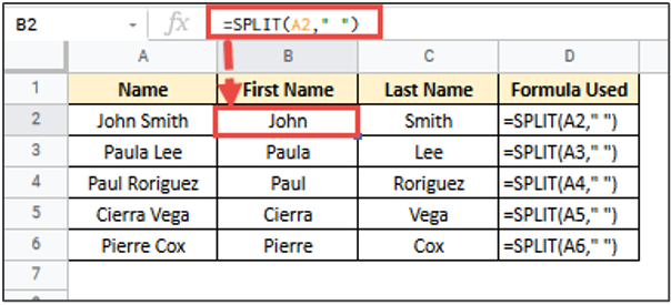
You can use the SPLIT function for lots of other cases too. For example, you can use it to separate a full address in a cell into street, city and Zip code. You could also use it to split an email address into its constituent parts. The possibilities are endless.
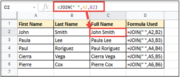
In contrast to the SPLIT function, the JOIN function combines information in different strings (or columns) into a single string, by separating them with a delimiter. As such you an use this function when you have the first and last names in separate columns and you need to combine them to get full names, as shown below:
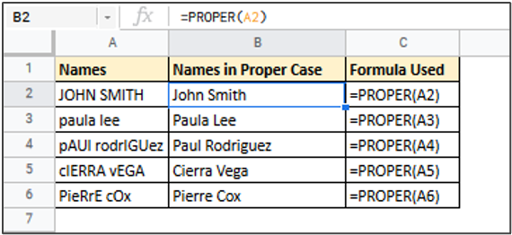
PROPER
Sometimes you might need to change the capitalization in the text to clean up or make your data look consistent. This is especially difficult to do when you want to specify titles, like book or movie names.
You can use the Google Sheets PROPER function to get this done. This function capitalizes the first letter of every word in the given string, as shown below:
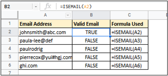
ISEMAIL
Finally, if you’re running a business you obviously need to work with emails. A major part of client interaction involves extracting email addresses from inputs received through forms.
You might have an opt-in form on your website that asks visitors for their email address. Most of the time you’ll find people either entering false email addresses or email addresses in the wrong format. It’s always smarter to filter out these false / invalid email addresses before saving them to your spreadsheet, to save you time and effort later on.
The ISEMAIL function is perfect for such scenarios. This function validates a given email address format and, in the process, helps identify which email addresses are likely to bounce, owing to an invalid format.
If the email address is valid the function returns a TRUE value, otherwise it returns a FALSE value.
Conclusion
So that was it! We gave you our top 10 spreadsheet formulas that can make you an Excel and Google Sheets pro, giving an effective edge to your business spreadsheets.
Of course this is not an exhaustive list and there’s a host of other useful Google Sheets formulas. However, start with these and then make your way up to more complex ones.
After all, there’s no end to learning, but you’ve got to start somewhere! Let this list be the starter kit that you need!